


Summary
This article presents a standardized technique to evaluate the navigation performance (position, velocity, and principal axes) of an airborne system and develop an efficient methodology to define the number of target data points to process during the planning phases of testing. This technique gave statistical credibility and rigor to the test while saving time and funds and with the minimum amount of data to achieve significant results.
Three units under test (UUTs) were used that underwent ground and flight tests alongside a reference system. The proposed methodology involved calculating the Pearson correlation coefficient to find intervals of random error. These intervals were used to pick out the data points to use for calculating error. For a more complete analysis, the error calculated using this methodology was shown alongside available data.
The difference between the two methods of calculating error was nearly negligible across all UUTs and time, space, and position information (TSPI) columns of interest, with multiple instances of 0% difference.
Introduction
Since its inception, engineers and scientists have continuously worked to enhance the accuracy and precision of global positioning system (GPS) and inertial navigation system (INS) technologies [1]. These efforts have focused on overcoming inherent system limitations and environmental challenges, enabling reliable performance in a wide range of applications. GPS and INS systems, while individually robust, are often integrated into hybrid configurations to capitalize on their complementary strengths. For example, embedded GPS and INS packages combine the long-term accuracy of GPS with the short-term stability of INS, allowing for multiple navigation modes and improved system redundancy [2–5]. This integration mitigates errors associated with each standalone system, such as GPS signal degradation in obstructed environments or INS drift over extended durations.
To further enhance performance, many navigation systems incorporate real-time error estimation algorithms. These algorithms leverage statistical models to quantify and correct for errors in position, velocity, and orientation during operation [6, 7]. By continuously refining their estimates, such systems provide users with more accurate and reliable navigation solutions. For instance, state-of-the-art error estimation techniques often utilize Kalman filtering or similar probabilistic approaches to fuse sensor data and predict system accuracy [8, 9].
Accuracy measurements for navigation systems are typically evaluated in the Earth-centered, Earth-fixed (ECEF) coordinate system, which defines errors in the X, Y, and Z directions as ∆Xi, ∆Yi, and ∆Zi , respectively. These errors can result from various sources, including signal multipath, atmospheric disturbances, and sensor noise. Quantifying these errors is critical for system validation, particularly in applications with stringent performance requirements, such as aviation and autonomous vehicle navigation. While numerous metrics exist for assessing navigation accuracy, two are commonly employed—spherical error probable (SEP) and root mean squared (RMS) error.
SEP provides a probabilistic measure of positional accuracy, defining the radius within which a certain percentage of positional estimates fall [10]. However, this article focuses on RMS, a metric that directly quantifies the average magnitude of errors in all three spatial dimensions. RMS offers a straightforward and comprehensive means of comparing system performance under various conditions.
When designing a test to evaluate GPS accuracy, a central question arises: “How much data is enough?” This question often sparks debate among stakeholders. Engineers and system developers, aiming to maximize statistical reliability, typically advocate for collecting as much data as possible. Conversely, financial analysts and project managers, focused on minimizing costs and resources, push for constraints on data collection efforts. Striking a balance between these competing priorities requires careful statistical planning during the test design phase. By incorporating foresight into the expected number of observations, it is possible to achieve a rigorous analysis without excessive resource expenditure.
One of the foundational statistical tools for addressing sample size requirements is the Student’s t-Distribution, a widely used approach for analyzing small datasets. This is particularly effective when the goal is to estimate the mean of a normally distributed population where the sample size is small and the population standard deviation is unknown [11]. A commonly cited rule of thumb suggests that a minimum of 30 data points is sufficient to utilize the t-Distribution effectively [12]. This threshold is rooted in the central limit theorem, which states that the sampling distribution of the mean approaches normality as the sample size increases, even if the underlying population distribution is not perfectly normal [13, 14]. For small samples, the t-Distribution provides a robust framework with well-defined properties, including n − 1 degrees of freedom and an expected mean of zero, variance of 1, and standard normal behavior, denoted as N ∼ (0,1).
However, determining the appropriate sample size involves more than adhering to arbitrary thresholds. The choice of 30 data points assumes that the data represent the population and that the chosen distribution accurately models the underlying behavior. If these assumptions are violated—such as when the data exhibit significant skewness, kurtosis, or outliers—additional considerations must be made [15, 16]. For example, heavily skewed distributions may require larger sample sizes to achieve reliable results, while data with outliers may necessitate robust statistical methods or preprocessing to mitigate their influence [17].
An equally critical aspect of sample size determination is defining what constitutes a valid data point. In GPS accuracy testing, a “data point” often corresponds to a discrete event or observation, such as a position fix or navigation update. The temporal and spatial resolution of these observations can significantly impact the test results. For instance, higher-frequency data collection may capture transient anomalies that lower-frequency sampling would miss, while excessive sampling may introduce redundancy without adding meaningful information [18]. Understanding these trade-offs is essential for ensuring that the collected data is sufficient and efficient for the intended analysis.
While many test designs rely on post-hoc statistical power analysis to validate results after data collection, this approach can be inefficient and costly. By integrating statistical planning into the test design process, planners can optimize data collection strategies, reduce resource consumption, and improve the overall reliability of their findings. Techniques such as power analysis, sensitivity analysis, and simulation-based methods can help refine sample size estimates and identify the minimum data requirements for achieving statistically significant results [19, 20].
Ultimately, the process of determining how much data is enough depends on a nuanced understanding of the statistical properties of the chosen methodology and the specific objectives of the test. This article aims to address these challenges by proposing a systematic approach to defining valid data points and evaluating sample size requirements in the context of GPS accuracy testing.
With a t-Distribution and the widely accepted target of 30 data points established, the next step is to clearly define what constitutes a valid sample. While the conceptual process of selecting data points may appear straightforward, the practical implementation often introduces complexities that can compromise the validity and reliability of results [21]. A data sample in GPS accuracy testing is typically tied to a specific event like a position update or navigation fix recorded during the operation of the system under test. However, the characteristics of these events—such as their temporal spacing, environmental conditions, or measurement noise—can significantly influence the outcomes of subsequent analyses.
A key challenge in this process is ensuring that the selected data points are representative of the underlying system behavior and relevant to the test objectives. For instance, if the test environment includes a mix of benign and degraded GPS conditions, the sampling strategy must account for this variability to avoid skewed results. Oversampling events in benign conditions could mask the system’s true limitations, while focusing disproportionately on degraded scenarios might inflate error metrics and lead to overly conservative conclusions. Additionally, the temporal distribution of data points plays a crucial role. Sampling intervals that are too short may introduce autocorrelation effects, where consecutive measurements are highly dependent, violating statistical independence assumptions [22]. Conversely, overly long intervals may fail to capture transient system behaviors critical to navigation performance evaluations.
In practice, many test planners adopt a comprehensive approach, utilizing all available data to calculate system accuracy. This approach often ensures that the results reflect the full spectrum of operating conditions encountered during the test. However, it can also lead to inefficiencies, such as processing redundant or irrelevant data, and may obscure critical insights into system performance under specific conditions. Moreover, relying on post-execution statistical power assessments, as is often the case, limits the ability to adapt data collection strategies in real-time, potentially compromising test outcomes [23].
To address these challenges, it is necessary to develop a systematic methodology for identifying valid data points. Such a methodology should consider the statistical properties of the data and the practical constraints of the test environment. For example, criteria for data selection might include thresholds for measurement uncertainty, filtering for specific environmental conditions, or stratification by navigation mode or operational phase. By incorporating these criteria into the test design process, planners can ensure that the selected data points provide meaningful insights while maintaining statistical rigor.
The assumption that 30 data points are sufficient for statistical significance also warrants scrutiny. Although this threshold is often a general rule of thumb, its applicability depends on several factors, including the underlying distribution of the data, the presence of outliers, and the desired level of confidence in the results [24–26]. For example, in cases where the data exhibit significant skewness or heavy tails, larger sample sizes may be required to achieve reliable estimates of central tendency and dispersion. Conversely, in well-controlled environments with low measurement noise, fewer data points may suffice to achieve the same level of statistical power [27].
The equations and concepts that underlie GPS and INS performance evaluations have been extensively applied in ground [28, 29] and airborne [30] systems, serving as the basis for establishing their suitability as reference systems. These efforts have culminated in developing highly accurate and well-characterized navigation systems, many of which remain benchmarks in the field [31].
However, a critical question often overlooked in these applications is what methodology is used to select the data points that form the basis of performance evaluations. While it is common practice to calculate the three-dimensional (3-D) error using all available data, this approach, while comprehensive, is not without drawbacks. Processing large datasets indiscriminately can lead to inefficiencies in terms of computational resources and test planning efforts, particularly when cost and time constraints are significant.
In specialized fields like navigation performance testing, where technical applications are highly specific, much of the expertise and methodologies is often passed down informally through experience rather than systematically documented. This reliance on institutional knowledge can create challenges in maintaining consistency and rigor, particularly when personnel turnover results in the loss of statistical analysis subject matter experts. As such, the development of a standardized, repeatable methodology for test planning is not just beneficial but essential for sustaining high standards within the testing community.
The traditional approach of leveraging all available data for analysis undoubtedly ensures that performance metrics represent the test conditions. However, this exhaustive approach can obscure opportunities to optimize the testing process, especially during the planning phase. A more efficient strategy involves defining what constitutes a valid data point in the context of the test objectives and using this definition to estimate the minimum sample size required for statistically significant results. By narrowing the scope to a subset of data that is representative and relevant, test planners can achieve dual goals of maintaining statistical rigor and reducing unnecessary resource expenditures.
This article proposes a novel methodology aimed at addressing these challenges, particularly by moving beyond the traditional reliance on Student’s t-Distribution assumptions. While the t-Distribution provides a robust framework for estimating population parameters under certain conditions, its utility in practical test planning is limited when the criteria for data selection and the characteristics of the dataset are poorly defined. By incorporating a systematic process for identifying valid data points, grounded in statistical tools like error interval calculations and correlation analyses, this methodology enables test planners to answer the critical question of how much data is enough with greater precision.
The remainder of this article details the development and application of this methodology, illustrating its potential to streamline the planning phase of navigation performance tests. The proposed approach offers a way to predefine data collection requirements that ensures efficiency and reliability, ultimately supporting the broader objective of delivering rigorous and cost-effective evaluations of GPS and INS systems.
Methodology
This section depicts the bulk purpose and focus of this article by presenting the approach and technique principles that were applied to flight test data.
Data Characteristics
TSPI was collected at the default data rates for each component: 1 Hz for GPS and 10 Hz for INS. These data sets were derived from multiple UUTs, manufactured by different vendors, and deployed on a fixed-wing, turboprop transport aircraft. The aircraft, modified for military testing, could carry cargo and personnel while supporting research and development evaluations of the onboard navigation systems. (Specifics beyond this are intentionally omitted for security reasons and to keep the emphasis of this article on the proposed process.)
The characteristics of the tests performed on each UUT in ground-based and airborne environments under varying conditions are shown in Table 1 and include the hours of ground test/flight tests, benign or degraded environments, range of velocity and position, and flight time in a degraded environment for 85 hours of testing across three different UUTs.
Table 1. Demographics of Flight Test Data From Three UUTs Flown on the Same Aircraft Across Multiple Sorties (Source: N. Ruprecht)
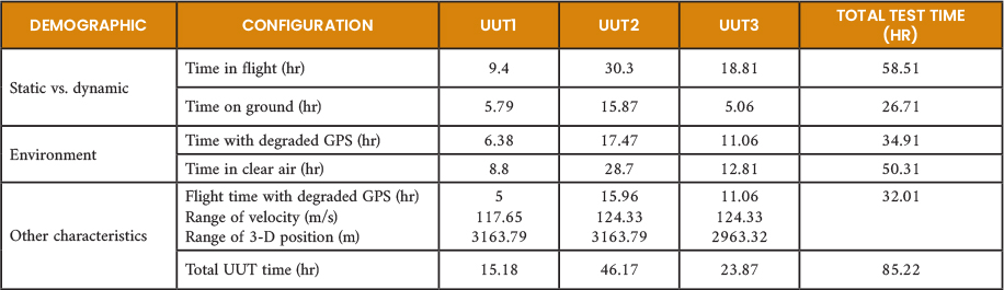
Each TSPI dataset consisted of 10 distinct columns: VX, VY, VZ (velocity components), PX, PY, PZ (ECEF position components), roll, pitch, yaw, and time. Here, P represents the ECEF positions along the three Cartesian axes, while yaw describes the rotation of the body axis. The datasets were intentionally standardized across UUTs to maintain consistency in comparisons.
The Ultra-High Accuracy Reference System (UHARS), built and maintained by the 746th Test Squadron (746 TS) at Holloman Air Force Base (AFB), NM, served as the standard reference system for these evaluations. UHARS is regarded for its ability to deliver highly precise positional and navigational data, even in challenging environments, making it an ideal benchmark for assessing the performance of emerging navigation systems. A critical characteristic of a reference system is its inherent accuracy and precision relative to the UUT. For robust testing, it is generally accepted that the reference system’s accuracy should exceed that of the UUT by at least an order of magnitude. This ensures that the reference system’s contribution to overall error is negligible when quantifying the performance of the UUT.
The technical justification for this rule of thumb is rooted in the propagation of uncertainty during error calculations. If the reference system’s error approaches the error of the UUT, it becomes challenging to differentiate between the inherent inaccuracies of the UUT and the limitations of the reference system itself [32, 33]. By maintaining an accuracy margin of 10:1, the reference system effectively isolates the UUT’s performance characteristics.
For instance, if the reference system’s positional accuracy is ~1 cm, it can reliably assess a UUT with positional errors near 10 cm or greater without introducing significant ambiguity into the results. The referenced “10× accuracy rule” is also rooted in practical testing heuristics, where the reference system is expected to be an order of magnitude more accurate than the system under test. This is also known as the Gagemaker’s Rule or Rule of Ten. It has been associated with military standards like MIL-STD-120 released in 1950 but has shifted to a 25% tolerance and is becoming increasingly challenging to maintain in all cases [34].
Additionally, ISO/IEC 17025, a global standard for testing and calibration laboratories, highlights the need for traceability and rigorous uncertainty analysis to ensure that the reference system’s errors do not compromise the integrity of the test results [35]. By maintaining this high level of accuracy, UHARS ensures that observed deviations during testing can be confidently attributed to the performance of the UUTs rather than errors introduced by the reference system. This approach upholds the statistical credibility and reliability required for evaluating navigation system performance, particularly in environments where precision is critical.
Proposed Technique
There are multiple sources of errors related to GPS. These errors are made up of time-correlated and nontime-correlated components [36, 37]. Inertial systems also have correlations due to their inherent growth in inertial sensor error [38]. To characterize a system, the errors that are evaluated at a certain time should be uncorrelated (correlation coefficient zero) of any other [39, 40]. Note that this process requires the data to have zero correlation but not zero dependence, where correlation is the measure of linear dependence. Since the UUT and reference system will have similar distribution of errors for a given column and one does not affect or impact the other, the systems are assumed independent and identically distributed.
The overall process presented to evaluate the navigation performance of airborne systems follows four steps:
- Align, interpolate, and clip data so that data analyzed records the UUT and reference system.
- Find correlation coefficient for k number of lags and save the first occurrence k of zero autocorrelation (ZAC) for each column of interest.
- Calculate RMS error at modulus intervals of previous step between the UUT and corresponding reference data point.
- If the target system specification (population mean) is known, use (a). Otherwise, use (b), where (a) runs a hypothesis test given these sample errors, target specification, standard deviation, and number of samples collected at those intervals (thus saving and presenting the hypothesis test result and corresponding t-statistic and one-sided p-value for each column of interest) and (b) creates a single tailed, upper bound confidence interval for these sample errors, number of samples collected, and chosen α for each column of interest. Also calculated is the RMS error (Step 3) using all available data to show side-by-side comparison of techniques and that the two are comparable.
Algorithm 1 (Figure 1) is used to preprocess the TSPI data collected during each test. If the UUT and reference system are not precisely synchronized for recording and sample at different GPS times, this script aligns the two sets of data by finding the minimum error between the time columns and assigning that row to the final reference variable to be used. If the sampling frequencies of the two systems are different, the script still accounts for this using minimum error and may then list the same row multiple times. The “while” loop is used in case the system recording starts or ends before/after the other system. It will log the index for the first time the two variables show alignment and the last, therefore clipping the UUT and ref variables.
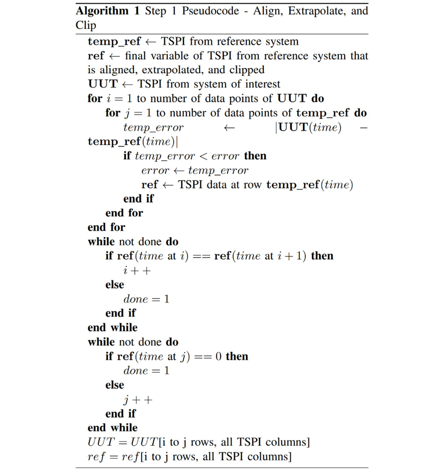
Figure 1. Algorithm 1 (Source: N. Ruprecht).
After preprocessing and data cleaning, each column of interest is compared to itself to check for correlation (autocorrelation). Each index is compared to every other as the data is shifted by its entire length to find the Pearson correlation coefficient for each lag. Given measurements Y1, Y2, …, YN at time X1, X2, …, XN, the lag k autocorrelation function is defined in Equation 1 as follows:
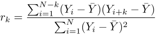 . (1)
. (1)
Algorithm 2 (Figure 2) finds the coefficient of each data sample compared to a shifted vector (lag) of itself using a Python function that utilized this equation. There may be multiple instances of zero correlation between data points and therefore multiple intervals that can be used to build a data array. To have the least amount of time between points, this script looks for the first occurrence of zero correlation for each TSPI column.
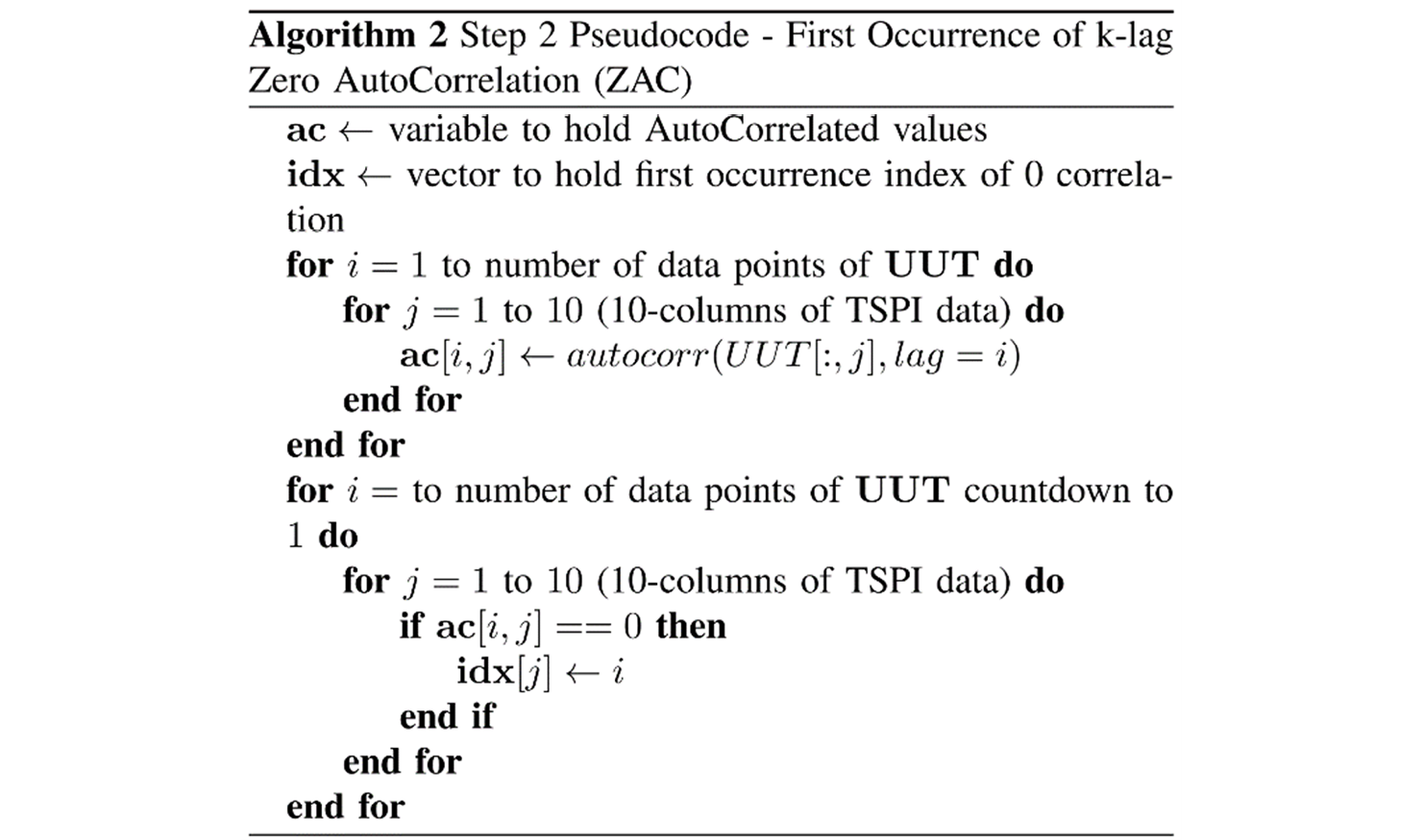
Figure 2. Algorithm 2 (Source: N. Ruprecht).
After the smallest interval between uncorrelated data, Algorithm 3 (Figure 3) goes back through the UUT data to calculate error. Using the modulo function, if i is a multiple of the index for a given column, that data point in UUT is used against the reference system at that same point in time (or closest to referring to Algorithm 1 in aligning). With arrays of absolute errors, the dataset can now be analyzed knowing its errors are random or uncorrelated. In this case, the RMS, standard deviation, and number of data points of each column (N ) are saved to Stats.
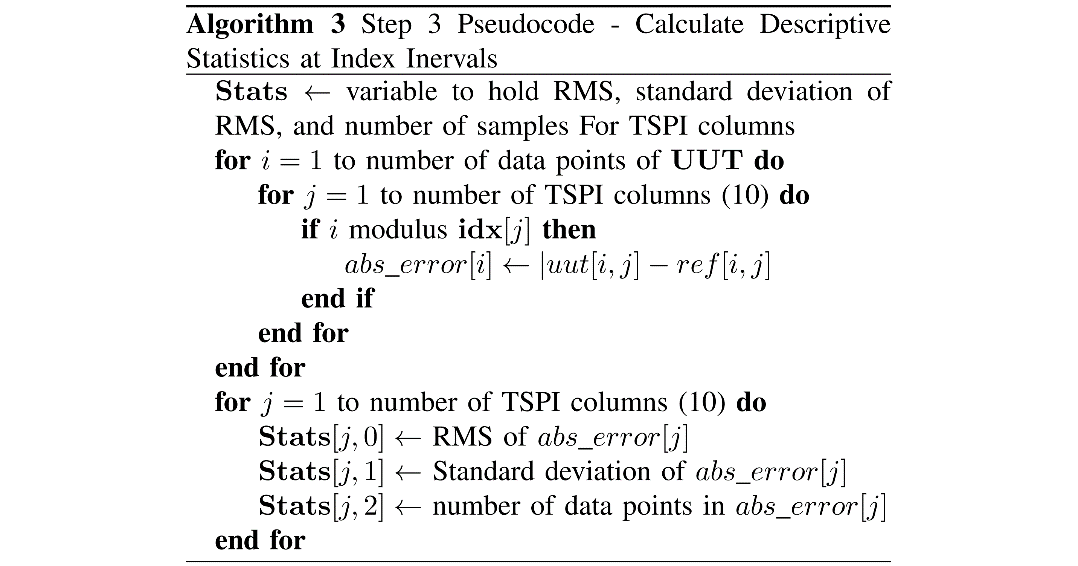
Figure 3. Algorithm 3 (Source: N. Ruprecht).
Finally, Algorithm 4 (Figure 4) shows the final piece of characterizing the UUT.
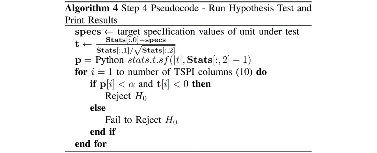
Figure 4. Algorithm 4 (Source: N. Ruprecht).
Using the Stats variable, a single-mean, t-statistic is calculated based on error as defined by Equation 2, where x is the sample mean error given by the column’s RMS, s is the sample standard deviation, N is the number of samples used, and µ is the population mean error given by the target specification RMS for each column:
![]() . (2)
. (2)
With a t-statistic, the single-sided p-value can be determined using a Python function in the statistics library. With these two knowns, a hypothesis test is run with the null and alternative defined as H0: x ≥ µ and Ha: x < µ, with rejecting H0 if p < α and t < 0, where α = 0.05 in this case. The reason for this order is to have a starting assumption that the UUT error is too great or considered “out of spec.” When using a hypothesis test, the null hypothesis cannot be “accepted”—only “fail to reject” the null. The UUT would rather be proven to be within specification by rejecting the current null hypothesis, as opposed to fail to reject the idea of it being within specification. Failing to reject the null hypothesis can be interpreted as meaning that the UUT has a greater error than required or that not enough data was collected to statistically prove the error is less.
Results and Discussion
Raw errors and results are summarized next. Figure 5 shows the difference in the ratio between the techniques used. The Y-axis on the left corresponds to the difference comparing calculated RMS error when looking at uncorrelated data points vs. error and using all available data. Due to the different scales of magnitude for each TSPI column unit, a ratio difference was used to standardize an output for visual representation’s sake. The Y-axis on the right aligns with the number of samples used for each UUT and TSPI column to achieve a statistically significant (p-value <0.05) ZAC for RMS calculation and evidence-based decision making in the number of data points needed for each column of interest.
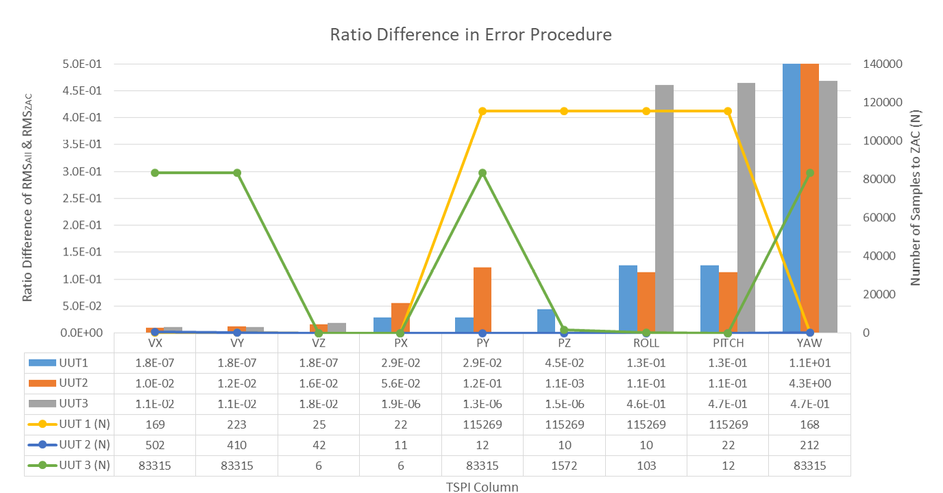
Figure 5. Calculated RMS Using All Available Data (RMSAll) vs. Calculated RMS With Uncorrelated Values or ZAC (RMSZAC) (Source: N. Ruprecht).
The figure combines two thought processes—the difference in calculated error along the left y-axis and the number of data points it took to get a statistically significant uncorrelated error along the right y-axis. For nearly all TSPI columns and UUTs, the difference in error calculation technique is near zero and therefore comparable. The few instances where the differences were larger were consistent across UUTs or TSPI columns. Another interesting finding is how small N can be and still have statistically significant results. Where 30 samples are a good rule of thumb, this shows that conclusions can be drawn with less while, at times, more is necessary. If a representative dataset is available, this methodology can be used to estimate the target number of samples and required test time more empirically than as a rule of thumb. Overall, negligible difference leans into the purpose of this article that asserts the methodology presented can be used so that the tester can speak definitively about how much data, flight time, and sorties will be required well before the test execution itself.
When evaluating datasets after the fact, the aircraft could enter and exit degraded environments so that the entire flight is broken down to intervals of interest. Here, the results of an entire flight can be the sum of its parts such that using this methodology on each part will have the same conclusion as running on the entire flight. An interesting outcome to see is how much the interval and number of samples used varies for the same flight. Looking more into the flight profile, it intuitively speaks to these values.
Since correlation is inversely proportional to the variance of data being used, a repetitive flight such as racetracks or orbits will require more data to have temporal separation to decorrelate. In contrast, columns with higher variance saw the correlation coefficient approach zero much earlier. Variance also plays directly into the results of the hypothesis test. With a higher variance in the flight profile, more data points are collected due to a smaller time interval before decorrelation occurs. This almost equates to a lower variance in the flight profile, therefore collecting less data due to a larger interval. The t-statistic is therefore mainly determined by the RMS error.
Conclusions
This study presents a foundational methodology for determining the necessary amount of data required to achieve statistically significant navigation performance evaluation results. While this approach has not yet been extensively validated against surveyed systems or multiple reference standards, its potential impact on test planning and execution is evident. The key contribution of this work is demonstrating that by leveraging the correlation coefficient, an optimal sample size can be determined for error estimation without relying on traditional heuristics such as the 30-sample rule.
The results presented here indicate that for nearly all TSPI parameters and UUTs, the calculated root mean squared error (RMS) using all available data (RMSAll) and the RMS derived from statistically independent data points (RMSZAC) yield nearly identical values. This suggests that decorrelating the dataset before error computation does not introduce significant bias and can be a viable alternative for test planners. Moreover, the findings highlight that the number of required samples can be highly variable, depending on the variance and structure of the test flight profile. Repetitive maneuvers, such as racetracks or orbits, introduce greater temporal correlation and therefore require a larger dataset to achieve statistical independence, whereas more dynamic flight profiles with higher variance can decorrelate more quickly.
A key implication of this methodology is its ability to assist in defining the required test duration and sortie count before execution. By applying this method to preexisting UUT datasets—without necessitating a reference system—engineers can estimate the minimum number of independent samples needed. This enables more precise test planning, ensuring that sufficient data is collected without unnecessary resource expenditure. Given the constraints of flight test programs, including fuel limitations, airspace availability, and cost considerations, this methodology provides an empirical, data-driven approach to optimizing test efficiency.
Recommendations
Future work should focus on validating the method presented here against independently surveyed reference systems and assessing its applicability across a wider range of navigation technologies and test conditions. Incorporating additional error sources like measurement noise and sensor drift into the model could further refine the accuracy of the predicted sample size. By establishing a standardized process for determining statistically significant test durations, this methodology can possibly improve the rigor and efficiency of navigation system evaluations across military and civilian applications.
Acknowledgments
The authors would like to acknowledge and thank the 746 TS and 704th Test Group for providing administrative oversight and support to maintain high standards of test rigor and approachability to improve capabilities for the test community. While specifics could not be disclosed for security reasons, the squadron’s and group’s commitment allowed free flow of thought and communication that was invaluable for improvement.
References
- Blewitt, G. “Basics of the GPS Technique: Observation Equations.” Geodetic Applications of GPS, pp. 10–54, 1997.
- Falco, G., G. A. Einicke, J. T. Malos, and F. Dovis. “Performance Analysis of Constrained Loosely Coupled GPS/INS Integration Solutions.” Sensors, vol. 12, no. 11, pp. 15983–16007, 2012.
- Li, Y., J. Wang, C. Rizos, P. Mumford, and W. Ding. “Low-Cost Tightly Coupled GPS/INS Integration Based on a Nonlinear Kalman Filtering Design.” Proceedings of ION National Technical Meeting, pp. 18–20, 2006.
- Wendel, J., J. Metzger, R. Moenikes, A. Maier, and G. Trommer. “A Performance Comparison of Tightly Coupled GPS/INS Navigation Systems Based on Extended and Sigma Point Kalman Filters.” Proceedings of the 18th International Technical Meeting of the Satellite Division of The Institute of Navigation (ION GNSS 2005), pp. 456–466, 2005.
- Kim, H.-S., S.-C. Bu, G.-I. Jee, and C. G. Park. “An Ultra-Tightly Coupled GPS/INS Integration Using Federated Kalman Filter.” Proceedings of the 16th International Technical Meeting of the Satellite Division of The Institute of Navigation (ION GPS/GNSS 2003), pp. 2878–2885, 2003.
- Xu, B., Y. Wang, and X. Yang. “Navigation Satellite Clock Error Prediction Based on Functional Network.” Neural Processing Letters, vol. 38, no. 2, pp. 305–320, 2013.
- Ober, P. B. “Integrity Prediction and Monitoring of Navigation Systems,” 2004.
- Misra, P., and P. Enge. Global Positioning System: Signals, Measurements and Performance. Second edition, vol. 206, 2006.
- Diggelen, F. GNSS Accuracy: Lies, Damn Lies, and Statistics. Vol. 9, pp. 41–45, January 2007.
- Schulte, R. J., and D. W. Dickinson. “Four Methods of Solving for the Spherical Error Probable Associated With a Three-Dimensional Normal Distribution.” Technical report, U.S. Air Force Missile Development Center, Holloman Air Force Base (AFB), NM, 1968.
- Hogg, R. V., E. A. Tanis, and D. L. Zimmerman. Probability and Statistical Inference. Upper Saddle River, NJ: Pearson/Prentice Hall, 2010.
- Van Belle, G. Statistical Rules of Thumb. John Wiley and Sons, 2011.
- Rosenblatt, M. “A Central Limit Theorem and a Strong Mixing Condition.” Proceedings of the National Academy of Sciences, vol. 42, no. 1, pp. 43–47, 1956.
- Singh, A. S., and M. B. Masuku. “Sampling Techniques and Determination of Sample Size in Applied Statistics Research: An Overview.” International Journal of Economics, Commerce and Management, vol. 2, no. 11, pp. 1–22, 2014.
- Carling, K. “Resistant Outlier Rules and the Non-Gaussian Case.” Computational Statistics and Data Analysis, vol. 33, no. 3, pp. 249–258, 2000.
- Iacobucci, D., S. Roman, S. Moon, and D. Rouzies. “A Tutorial on What to Do With Skewness, Kurtosis, and Outliers: New Insights to Help Scholars Conduct and Defend Their Research.” Psychology and Marketing, 2025.
- Wan, X., W. Wang, J. Liu, and T. Tong. “Estimating the Sample Mean and Standard Deviation from the Sample Size, Median, Range and/or Interquartile Range.” BMC Medical Research Methodology, vol. 14, pp. 1–13, 2014.
- Sahasranand, K., F. C. Joseph, H. Tyagi, G. Gurrala, and A. Joglekar. “Anomaly-Aware Adaptive Sampling for Electrical Signal Compression.” IEEE Transactions on Smart Grid, vol. 13, no. 3, pp. 2185–2196, 2022.
- Nguyen, A.-T., S. Reiter, and P. Rigo. “A Review on Simulation Based Optimization Methods Applied to Building Performance Analysis.” Applied Energy, vol. 113, pp. 1043–1058, 2014.
- Razavi, S., A. Jakeman, A. Saltelli, C. Prieur, B. Iooss, E. Borgonovo, E. Plischke, S. L. Piano, T. Iwanaga, W. Becker, et al. “The Future of Sensitivity Analysis: An Essential Discipline for Systems Modeling and Policy Support.” Environmental Modelling and Software, vol. 137, p. 104954, 2021.
- Fielding, S., P. Fayers, and C. R. Ramsay. “Analysing Randomised Controlled Trials With Missing Data: Choice of Approach Affects Conclusions.” Contemporary Clinical Trials, vol. 33, no. 3, pp. 461–469, 2012.
- Griffith, D. A., and R. E. Plant. “Statistical Analysis in the Presence of Spatial Autocorrelation: Selected Sampling Strategy Effects.” Stats, vol. 5, no. 4, pp. 1334–1353, 2022.
- Karunarathna, I., P. Gunasena, T. Hapuarachchi, and S. Gunathilake. “The Crucial Role of Data Collection in Research: Techniques, Challenges, and Best Practices.” UVA Clinical Research, pp. 1–24, 2024.
- Wang, H., and Z. Abraham. “Concept Drift Detection for Streaming Data.” The 2015 International Joint Conference on Neural Networks (IJCNN), pp. 1–9, IEEE, 2015.
- Osborne, W., and A. Overbay. “The Power of Outliers (and Why Researchers Should Always Check for Them).” Practical Assessment, Research, and Evaluation, vol. 9, no. 1, p. 6, 2019.
- Morey, R. D., R. Hoekstra, J. N. Rouder, M. D. Lee, and E.-J. Wagenmakers. “The Fallacy of Placing Confidence in Confidence Intervals.” Psychonomic Bulletin and Review, vol. 23, pp. 103–123, 2016.
- Schwarz, N., F. Strack, A. Gelman, S. M. van Osselaer, and J. Huber. “Commentaries on Beyond Statistical Significance: Five Principles for the New Era of Data Analysis and Reporting.” Journal of Consumer Psychology, vol. 34, no. 1, pp. 187–195, 2024.
- Yang, J.-S. “Travel Time Prediction Using the GPS Test Vehicle and Kalman Filtering Techniques.” Proceedings of the 2005 American Control Conference, pp. 2128–2133, IEEE, 2005.
- Hong, S., M. H. Lee, S. H. Kwon, and H. H. Chun. “A Car Test for the Estimation of GPS/INS Alignment Errors.” IEEE Transactions on Intelligent Transportation Systems, vol. 5, no. 3, pp. 208–218, 2004.
- Brown, A., and Y. Lu. “Performance Test Results of an Integrated GPS/MEMS Inertial Navigation Package.” Proceedings of ION GNSS, vol. 2004, Citeseer, 2004.
- Amt, H., and J. F. Raquet. “Flight Testing of a Pseudolite Navigation System on a UAV.” U.S. Air Force Institute of Technology: ION Conference, 2007.
- Stratton, A. “Flight Test Criteria for Qualification of GPS-Based Positioning and Landing Systems.” Proceedings of the 22nd International Technical Meeting of the Satellite Division of The Institute of Navigation (ION GNSS 2009), pp. 1610–1618, 2009.
- Jacobs, T. “Challenges of Moving a Mixed Technology Manual Test Setup Into an Automated Environment.” 2024 IEEE AUTOTESTCON, pp. 1–5, IEEE, 2024.
- Defense Logistics Agency. Gage Inspection. MIL-STD-120, 1950.
- International Organization for Standardization (ISO) and International Electrotechnical Commission (IEC). General Requirements for the Competence of Testing and Calibration Laboratories. ISO/IEC 17025:2017, 2017.
- Tiwari, R., M. Arora, and A. Kumar. “An Appraisal of GPS Related Errors.” Geospatial World, vol. 5, no. 9, 2000.
- Dmitrieva, K., P. Segall, and A. Bradley. “Effects of Linear Trends on Estimation of Noise in GNSS Position Time Series.” Geophysical Journal International, p. ggw391, 2016.
- Wall, J. H., and D. M. Bevly. “Characterization of Inertial Sensor Measurements for Navigation Performance Analysis.” Proceedings of the 19th International Technical Meeting of the Satellite Division of The Institute of Navigation (ION GNSS 2006), pp. 2678–2685, 2006.
- Mari, D. D., and S. Kotz. “Correlation and Dependence.” World Scientific, 2001.
- Szekely, G. J., M. L. Rizzo, N. K. Bakirov, et al. “Measuring and Testing Dependence by Correlation of Distances.” The Annals of Statistics, vol. 35, no. 6, pp. 2769–2794, 2007.
Biographies
Nathan A. Ruprecht is a U.S. Air Force (USAF) active-duty engineer in navigation systems and nuclear physics and assistant director of operations at the 21st Surveillance Squadron, Air Force Technical Applications Center, deploying as a scientist. Previously a flight test engineer at the 746 TS, he is in the process of transitioning to the National Air and Space Intelligence Center. Dr. Ruprecht holds a B.S. and M.S. in electrical engineering from the University of North Texas and a Ph.D. in biomedical engineering from the University of North Dakota.
Elisa N. Carrillo is a systems engineer with Raytheon Technologies, with expertise in validation and verification. Her research interests include cross-functional communication as a key element of systems integration, test, and validation. Ms. Carrillo holds a B.S. in mechanical engineering from the University of Texas at El Paso and is studying for her M.S. in systems engineering at Embry-Riddle Aeronautical University.
Loren E. Myers is an active-duty flight test engineer at the Air Dominance Combined Test Force, Edwards AFB, CA, where he executes flight test operations for the F-22A Raptor. His experience includes National Security Space Launch operations and developmental test of navigation systems at the Central Inertial and GPS Test Facility at Holloman AFB. Capt. Myers holds a B.S. in computer engineering from Washington State University, an M.S. in electrical engineering from the Air Force Institute of Technology, and an M.S. in experimental flight test engineering from the USAF Test Pilot School.